Previous Chapter: Convolutional Neural Network
Next Chapter: Distributed Mode
Recurrent Neural Network and (LSTM)
Following part is an introduction to recurrent neural networks and LSTMs quoted from this great article.
Introduction to Recurrent Neural Network
Recurrent Neural Network
Humans don’t start their thinking from scratch every second. As you read this essay, you understand each word based on your understanding of previous words. You don’t throw everything away and start thinking from scratch again. Recurrent neural networks are deep learning networks addressing this issue. They have loops in them, allowing information to persist.
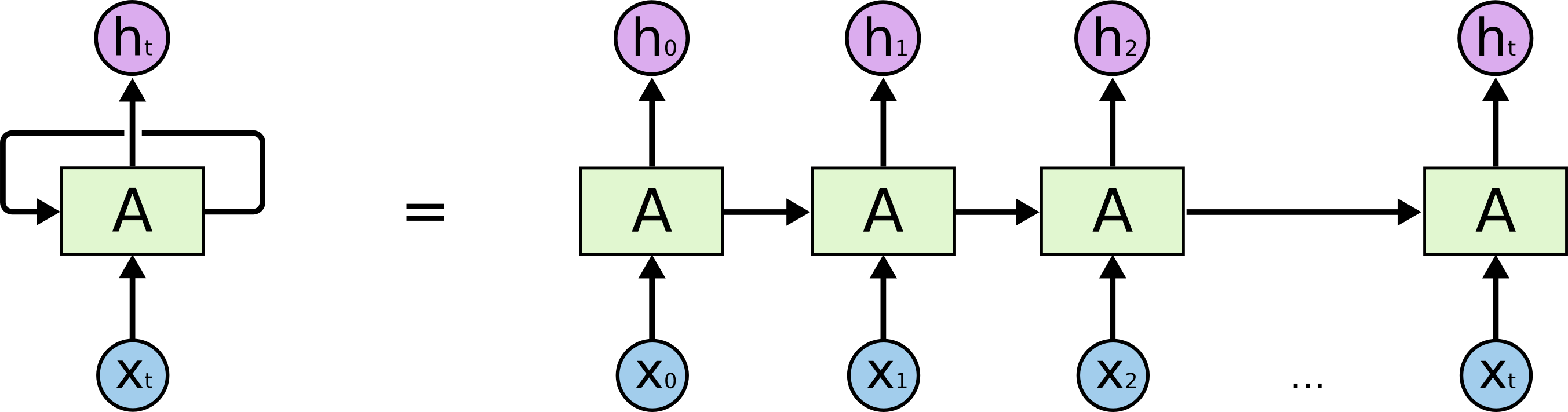
This chain-like nature reveals that recurrent neural networks are intimately related to sequences and lists. They’re the natural architecture of neural network to use for such data. RNNs have been successfly applied to a variety of problems: speech recognition, language modeling, translation, image captioning.
A Major Problem in RNN
Consider trying to predict the last word in the text “I grew up in France… I speak fluent French.” Recent information suggests that the next word is probably the name of a language, but if we want to narrow down which language, we need the context of France, from further back. It’s entirely possible for the gap between the relevant information and the point where it is needed to become very large.
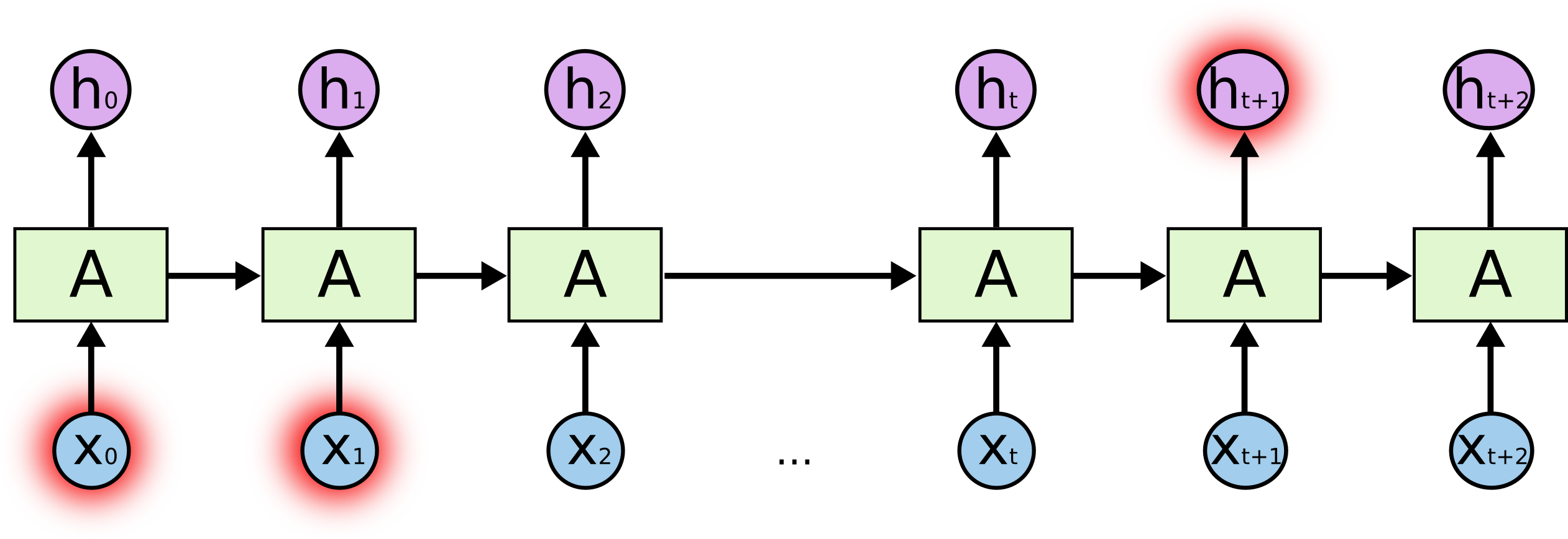
Unfortunately, as that gap grows, RNNs become unable to learn to connect the information.
LSTM Network
Long Short Term Memory networks – usually just called “LSTMs” – are a special kind of RNN, capable of learning long-term dependencies. They were introduced by Hochreiter & Schmidhuber (1997), and were refined and popularized by many people in following work.1 They work tremendously well on a large variety of problems, and are now widely used.
LSTMs are explicitly designed to avoid the long-term dependency problem. Remembering information for long periods of time is practically their default behavior, not something they struggle to learn!
All recurrent neural networks have the form of a chain of repeating modules of neural network. In standard RNNs, this repeating module will have a very simple structure, such as a single tanh layer.
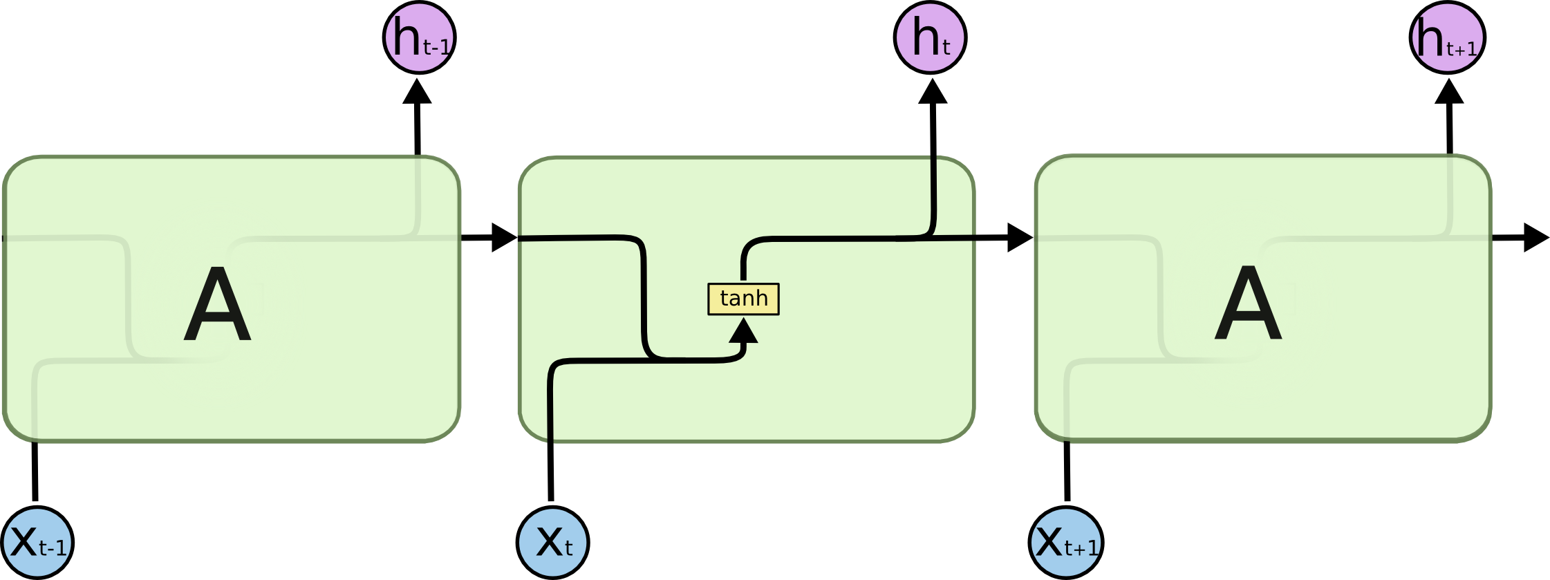
LSTMs also have this chain like structure, but the repeating module has a different structure. Instead of having a single neural network layer, there are four, interacting in a very special way.

In the above diagram, each line carries an entire vector, from the output of one node to the inputs of others. The pink circles represent pointwise operations, like vector addition, while the yellow boxes are learned neural network layers. Lines merging denote concatenation, while a line forking denote its content being copied and the copies going to different locations.
The key to LSTMs is the cell state, the horizontal line running through the top of the diagram.
The cell state is kind of like a conveyor belt. It runs straight down the entire chain, with only some minor linear interactions. It’s very easy for information to just flow along it unchanged.
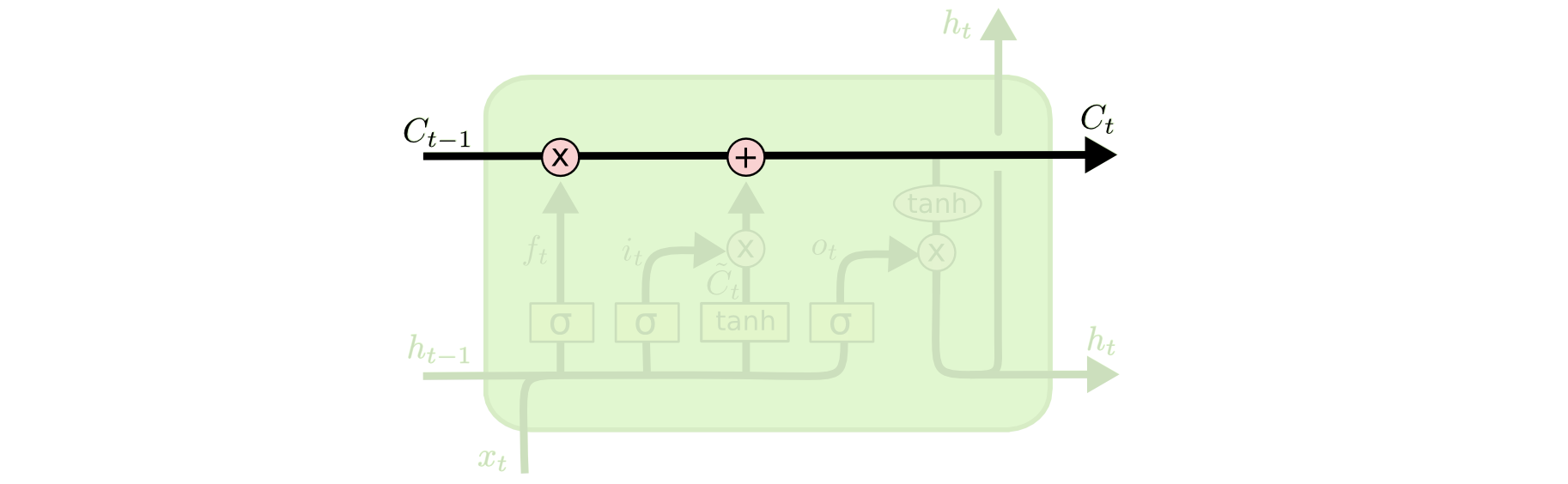
The LSTM does have the ability to remove or add information to the cell state, carefully regulated by structures called gates.
Gates are a way to optionally let information through. They are composed out of a sigmoid neural net layer and a pointwise multiplication operation.
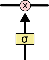
The sigmoid layer outputs numbers between zero and one, describing how much of each component should be let through. A value of zero means “let nothing through,” while a value of one means “let everything through!”
An LSTM has three of these gates, to protect and control the cell state.
Attention System
LSTMs were a big step in what we can accomplish with RNNs. It’s natural to wonder: is there another big step? A common opinion among researchers is: “Yes! There is a next step and it’s attention!” The idea is to let every step of an RNN pick information to look at from some larger collection of information. For example, if you are using an RNN to create a caption describing an image, it might pick a part of the image to look at for every word it outputs. In fact, Xu, et al. (2015) do exactly this – it might be a fun starting point if you want to explore attention! There’s been a number of really exciting results using attention, and it seems like a lot more are around the corner…
Attention isn’t the only exciting thread in RNN research. For example, Grid LSTMs by Kalchbrenner, et al. (2015) seem extremely promising. Work using RNNs in generative models – such as Gregor, et al. (2015), Chung, et al. (2015), or Bayer & Osendorfer (2015) – also seems very interesting. The last few years have been an exciting time for recurrent neural networks, and the coming ones promise to only be more so!
Exercise: Recurrent Neural Network
This is an exercise of Recurrent Neural Network.
Same as previous chapter
|
|
A little bit difference
To classify images using a recurrent neural network, we consider every image row as a sequence of pixels. Because MNIST image shape is 28*28px, we will then handle 28 sequences of 28 steps for every sample.
|
|
Training Steps
|
|
Weights and Biases
|
|
Graph
|
|
Summary
|
|
Run a Session
|
|
Previous Chapter: Convolutional Neural Network
Next Chapter: Distributed Mode