1. Introduction
An extension of principal component analysis(PCA) in the sense of approximating covariance matrix.
Goal
- To describe the covariance relationships among many variables in terms of a few underlying unobservable random variables, called factors.
- To reduce dimensions and solve the problem with n<p.
2. Orthogonal Factor Model(正交因子模型)
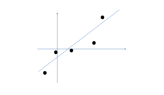
A Factor Analysis Example
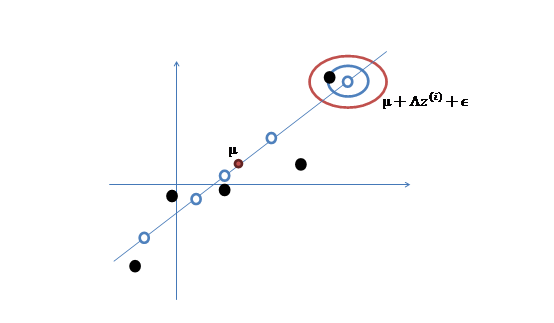
We have a training data $ X_{n \times p} $. Here is its scatter plot. $ y = a $
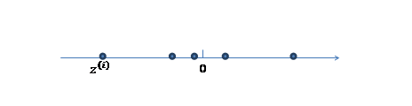
- Generate a k dimension variable $F \sim N_k(0,I)$
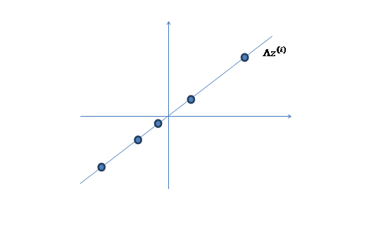
- There exists a transformation matrix $L \in R^{p \times k}$ which maps F into n dimension space: $LF$
- Add a mean $\mu$ on $LF$
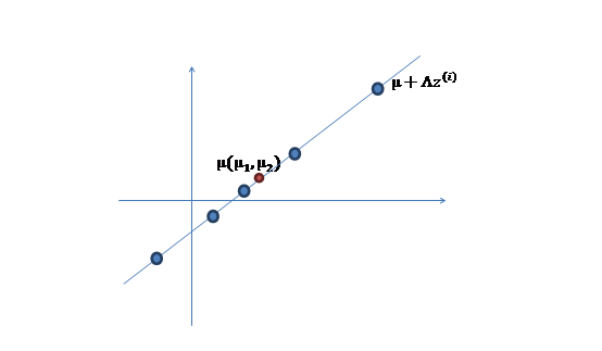
- For real instance has errors, add error $\epsilon_{p \times 1}$
$$X = LF+\mu + \epsilon$$
Factor Analysis Model
- Suppose $X \sim \Pi_p(\mu, \Sigma)$
- The factor model postulates that $X$ is linearly related to a few unobservable random variables $F_1,F_2,…,F_m$, called common factors(共同因子), through
where $L = (l_{ij})_{p \times m}$ is the matrix of factor loading(因子载荷), $l_{ij}$ is the loading of variable $i$ on factor $j$, $\epsilon = (\epsilon_1, . . . , \epsilon_p)′$, $\epsilon_i$ are called errors or specific factors(特殊因子).
- Assume:
$$E(F) = 0, cov(F) = I_m, $$
$$E(\epsilon) = 0, cov(\epsilon) = \psi_{p \times p} = diag(\varphi_1,.., \varphi_p)$$
$$cov(F, \epsilon) = E(F \epsilon ‘) = 0$$
Then
$$cov(X) = \Sigma_{p \times p} = LL’ + \psi$$
$$cov(X, F) = L_{p \times m}$$
If $cov(F) \ne I_m$, it becomes oblique factor model(斜交因子模型)
- Define the $i_{th}$ community(变量共同度,或公因子方差):
- Define the $i_{th}$ specific variance(特殊因子方差):
Ambiguity of L
- Let T be any m × m orthogonal matrix. Then, we can express
where $L^* = LT$, $F^* = T'F$
- Since $E(F^*) = 0$ , $cov(F^*) = I_{m}$ , $F^*$ and $L^*$ form another pair of factor and factor loading matrix.
After rotation, community $h_i^2$ doesn’t change.
3. Estimation
3.1 Principal Component Method
1) Get correlation matrix
$$\hat{Cor}(X) = \Sigma$$
2) Spectral Decompositions
$$\Sigma = \lambda_1\ e_1e_1’\ +\ …\ +\ \lambda_p\ e_pe_p’$$
3) Determine $m$
Rule of thumb: choose $m =\ \# \ of \{\lambda_j>1\}$
4) Estimation
$$\hat L = (\sqrt{\lambda_1}\ e_1,\ …\ ,\ \sqrt{\lambda_m}\ e_m)$$
$$\hat \psi = diag(\Sigma - LL’)$$
$$\hat h_i^2 = \sum_{j = 1}^m \hat l_{ij}^2$$The contribution to the total sample variance tr(S) from the first common factor is then(公共因子的方差贡献)
$$\hat l^2_{11} + ...+ \hat l^2_{p1} = (\sqrt{\hat \lambda_1}\hat e_1)'(\sqrt{\hat \lambda_1}\hat e_1) = \hat \lambda_1$$In general, the proportion of total sample variance(after standardization) due to the $j_{th}$ factor = $\frac{\hat \lambda_j}{p}$
3.2 Maximum Likelihood Method
1) Joint distribution:
$$ \begin{bmatrix} f\\ x \end{bmatrix} \sim N \begin{pmatrix} \begin{bmatrix} 0\\ \mu \end{bmatrix}, \begin{bmatrix} I & L'\\ L & LL' + \psi \end{bmatrix} \end{pmatrix}$$2) Marginal distribution:
$$x \sim N(\mu, LL’+\psi)$$
3) Conditional distribution:
$$\mu_{f|x} = L’(LL’+\psi)^{-1}(x-\mu)$$
$$\Sigma_{f|x} = I - L’(LL’+\psi)^{-1}L$$
4) Log likelihood:
$$l(\mu, L, \psi) = log \prod_{i=1}^n \frac{1}{(2 \pi)^{p/2}|LL’+\psi|} exp \left(-\frac{1}{2}(x^{(i)}-\mu)’(LL’+\psi)^{-1}(x^{(i)}-\mu) \right)$$
EM estimation
- E Step:
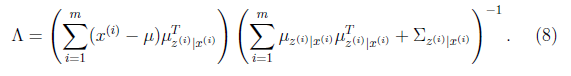
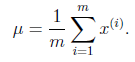
- M Step:
- Parameter Iteration:

$$\psi = diag(\Phi)$$
Get more detail on 【机器学习-斯坦福】因子分析(Factor Analysis)
4. Factor Rotation
An orthogonal matrix $T$, and let $L^* = LT$.
Goal: to rotate $L$ such that a ‘simple’ structure is achieved.
Kaiser (1958)’s varimax criterion(方差最大旋转) :
- Define $\widetilde l^*_ {ij} = \hat l^*_{ij}/h_i^2$
- Choose $T$ s.t.
5. Factor Scores
Weighted Least Squares Method
- Suppose that $\mu$, $L$, and $\psi$ are known.
- Then $X-\mu = LF + \epsilon \sim \Pi_p(0, \psi)$
$$\hat F = (L’ \psi ^{-1}L)^{-1}L’ \psi^{-1} (X-\mu)$$
Regression Method
From the mean of the conditional distribution of $F|X$ is $\mu_{f|x} = L’(LL’+\psi)^{-1}(x-\mu)$
$$\hat F = \hat E(F|X) = L’\Sigma^{-1}(X-\overline X)$$