Support Vector Machine

1 SVM

1.1 介绍

Support Vector Machine 支持向量机是一种机器学习算法。

给定一个训练集 \( S = \{ (x_i, y_i) \}_{i=1}^{m} \), 其中 \( x_i \in \mathbb{R}^n \) 并且 \( y_i \in \{ +1, -1 \} \), 图1展示了一个 SVM 需要解决的问题。我们标记 \( w \cdot x - b = 0 \) 为超平面， \( w \) 代表该超平面的向量。我们需要做的是找到能将 \( y_i=1 \) 的点和 \( y_i=-1 \) 的点分开的边际最大的超平面. 这就意味着 \( y_i(w \cdot x_i -b ) \geq 1 \)，对于所有 \( 1 \leq i \leq n \).

所以优化问题可以写成：

最大化

\[ \frac{2}{\|w\|} \]

这等价于最小化

\[ \frac{1}{2} \| w \|^2 \]

subject to \( y_i(w \cdot x_i - b) \geq 1 \) for all \( 1 \leq i \leq n \)

captionm

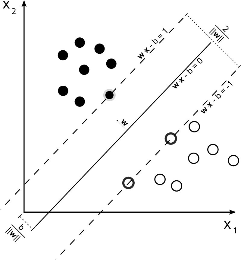
Figure 1: SVM

事实上，它可以被看作一个带有惩罚项的最小化损失问题。最终，我们希望找到以下问题的最小解

\[ \min_{w} \frac{\lambda}{2}\|w\|^2 + \frac{1}{m}\sum_{(x, y) \in S} \ell(w; (x, y)) \]

其中 λ 是正规化参数, \( \ell(w, (x, y)) \) 是 hinge 损失函数:

\[ \ell(w, (x, y)) = max\{0, 1-y \langle w, x \rangle \} \]

对于这一最优化问题，我们可以使用梯度下降算法来达到最小值。

目标函数为：

\[ f(w) = \frac{\lambda}{2}\|w\|^2 + \frac{1}{m}\sum_{(x_i, y_i) \in S}\ell(w; (x_i, y_i)) \]

所以，迭代 t 时的梯度为：

\[ \nabla_t = \lambda w_t - \frac{1}{m}\sum_{(x_i, y_i) \in S}\mathbb{1}[y_i \langle w, x_i \rangle < 1]y_i x_i \]

于是，我们可以更新 \( w \), 其中 \( \eta_t \) 是下降速度 \[ w_{t+1} \leftarrow w_t - \eta_t\nabla_t \]

1.2 SGD

从上一节我们可以看到每次迭代我们都需要所有的数据点来计算梯度。而当数据集变大后，无疑会耗费大量的计算时间。这就是为什么在大规模梯度下降算法中，我们总会使用 SGD（随机梯度下降）。SDG 在每次迭代时只使用一部分数据而不是全部，从而降低了计算量。

所以，现在目标函数变成了： \[ f(w, A_t) = \frac{\lambda}{2}\|w\|^2 + \frac{1}{k}\sum_{(x_i, y_i) \in A_t}\ell(w; (x_i, y_i)) \] where \( A_t \subset S \), \( |A_t| = k \). At each iteration, we takes a subset of data point.

然后梯度为： \[ \nabla_t = \lambda w_t - \frac{1}{k}\sum_{(x_i, y_i) \in A_t}\mathbb{1}[y_i \langle w, x_i \rangle < 1]y_i x_i \]

1.3 Pegasos and MLlib implementation

Pegasos 是 SVM 使用梯度下降算法的一种实现。Spark MLlib 也提供了 SVM 的梯度下降实现，于 Pegasos 稍有不同。主要是梯度的更新速度不同。

\[ w_{t+1} \leftarrow w_t - \eta_t\nabla_t \]

在 Pegasos 算法中, 更新速度为 \[ \eta_t = \frac{\alpha}{t\lambda} \]

而在 MLlib 中，为： \[ \eta_t = \frac{\alpha}{\sqrt{t}} \]

其中 α 是更新速度参数。

2 SGD in Spark

2.1 treeAggregate

Spark 来计算 SGD 的主要优势使可以分布式地计算梯度，然后将它们累加起来。在 Spark 中，这一任务是通过 RDD 的 treeAggregate 方法来完成的。 Aggregate 可被视为泛化的 Map 和 Reduce 的组合。 treeAggregate 的定义为

RDD.treeAggregate(zeroValue: U)(
      seqOp: (U, T) => U,
      combOp: (U, U) => U,
      depth: Int = 2): U

在此方法中有三个参数，其中前两个对我们更重要：

seqOp: 计算每隔 partition 中的子梯度
combOp: 将 seqOp 或上层 combOp 的值合并
depth: 控制 tree 的深度

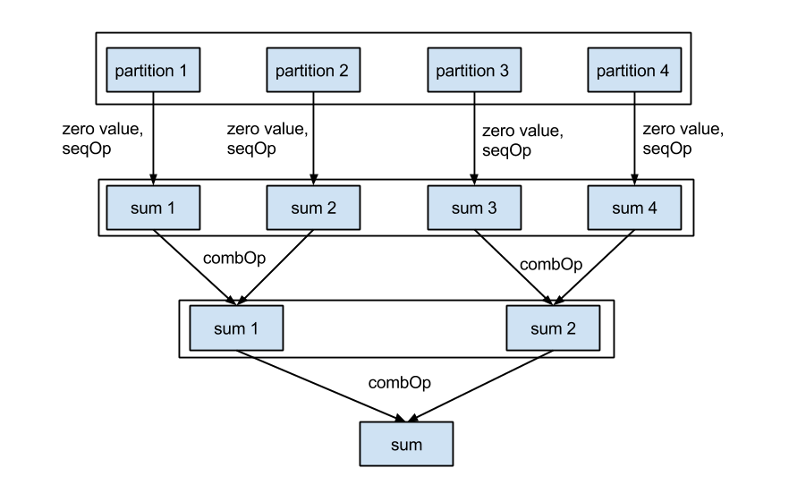
Figure 2: tree aggregate

2.2 实现

SGD 是一个求最优化的算法，许多机器学习算法都可以用 SGD 来求解。所以 Spark 对其做了抽象。

class SVMWithSGD private (
    private var stepSize: Double,
    private var numIterations: Int,
    private var regParam: Double,
    private var miniBatchFraction: Double)
  extends GeneralizedLinearAlgorithm[SVMModel] with Serializable {

  private val gradient = new HingeGradient()
  private val updater = new SquaredL2Updater()
  @Since("0.8.0")
  override val optimizer = new GradientDescent(gradient, updater)
    .setStepSize(stepSize)
    .setNumIterations(numIterations)
    .setRegParam(regParam)
    .setMiniBatchFraction(miniBatchFraction)

可以看到 SVMWithSGD 继承了 GeneralizedLinearAlgorithm ，并定义 optimizer 来确定如何获得优化解。而 optimizer 即是 SGD 算法的实现。正如上节所述，线性 SVM 实际上是使用 hinge 损失函数和一个 L2 惩罚项的线性模型，因此这里使用了 HingeGradient 和 SquaredL2Updater 作为 GradientDescent 的参数。

class HingeGradient extends Gradient {
  override def compute(data: Vector, label: Double, weights: Vector): (Vector, Double) = {
    val dotProduct = dot(data, weights)
    // Our loss function with {0, 1} labels is max(0, 1 - (2y - 1) (f_w(x)))
    // Therefore the gradient is -(2y - 1)*x
    val labelScaled = 2 * label - 1.0
    if (1.0 > labelScaled * dotProduct) {
      val gradient = data.copy
      scal(-labelScaled, gradient)
      (gradient, 1.0 - labelScaled * dotProduct)
    } else {
      (Vectors.sparse(weights.size, Array.empty, Array.empty), 0.0)
    }
  }

  override def compute(
      data: Vector,
      label: Double,
      weights: Vector,
      cumGradient: Vector): Double = {
    val dotProduct = dot(data, weights)
    // Our loss function with {0, 1} labels is max(0, 1 - (2y - 1) (f_w(x)))
    // Therefore the gradient is -(2y - 1)*x
    val labelScaled = 2 * label - 1.0
    if (1.0 > labelScaled * dotProduct) {
      axpy(-labelScaled, data, cumGradient)
      1.0 - labelScaled * dotProduct
    } else {
      0.0
    }
  }
}

/**
 * :: DeveloperApi ::
 * Updater for L2 regularized problems.
 *          R(w) = 1/2 ||w||^2
 * Uses a step-size decreasing with the square root of the number of iterations.
 */
@DeveloperApi
class SquaredL2Updater extends Updater {
  override def compute(
      weightsOld: Vector,
      gradient: Vector,
      stepSize: Double,
      iter: Int,
      regParam: Double): (Vector, Double) = {
    // add up both updates from the gradient of the loss (= step) as well as
    // the gradient of the regularizer (= regParam * weightsOld)
    // w' = w - thisIterStepSize * (gradient + regParam * w)
    // w' = (1 - thisIterStepSize * regParam) * w - thisIterStepSize * gradient
    val thisIterStepSize = stepSize / math.sqrt(iter)
    val brzWeights: BV[Double] = weightsOld.asBreeze.toDenseVector
    brzWeights :*= (1.0 - thisIterStepSize * regParam)
    brzAxpy(-thisIterStepSize, gradient.asBreeze, brzWeights)
    val norm = brzNorm(brzWeights, 2.0)

    (Vectors.fromBreeze(brzWeights), 0.5 * regParam * norm * norm)
  }
}

此节中, 1 展示了 GradientDescent 的主要执行逻辑。重复执行 numIterations 次以获得最终的 \( w \)。

首先, data.sample 通过 miniBatchFraction 取一部分样本. 然后使用 treeAggregate 。在 seqOp 中, gradientSum 会通过 axpy(y, b_x, c._1) 更新，如果 \( y\langle w, x \rangle < 1 \)，即分类错误。在 combOp 中, gradientSum 通过 c1._1 += c2._1 被集合起来。当获得 gradientSum 后, 我们就可以计算 step 和 gradient 了。最后, 我们使用 axpy(-step, gradient, weights) 更新 weights 。

GradientDescent 代码片断

while (!converged && i <= numIterations) {
  val bcWeights = data.context.broadcast(weights)
  // Sample a subset (fraction miniBatchFraction) of the total data
  // compute and sum up the subgradients on this subset (this is one map-reduce)
  val (gradientSum, lossSum, miniBatchSize) = data.sample(false, miniBatchFraction, 42 + i)
    .treeAggregate((BDV.zeros[Double](n), 0.0, 0L))(
      seqOp = (c, v) => {
	// c: (grad, loss, count), v: (label, features)
	val l = gradient.compute(v._2, v._1, bcWeights.value, Vectors.fromBreeze(c._1))
	(c._1, c._2 + l, c._3 + 1)
      },
      combOp = (c1, c2) => {
	// c: (grad, loss, count)
	(c1._1 += c2._1, c1._2 + c2._2, c1._3 + c2._3)
      })

  if (miniBatchSize > 0) {
    /**
     * lossSum is computed using the weights from the previous iteration
     * and regVal is the regularization value computed in the previous iteration as well.
     */
    stochasticLossHistory.append(lossSum / miniBatchSize + regVal)
    val update = updater.compute(
      weights, Vectors.fromBreeze(gradientSum / miniBatchSize.toDouble),
      stepSize, i, regParam)
    weights = update._1
    regVal = update._2

    previousWeights = currentWeights
    currentWeights = Some(weights)
    if (previousWeights != None && currentWeights != None) {
      converged = isConverged(previousWeights.get,
	currentWeights.get, convergenceTol)
    }
  } else {
    logWarning(s"Iteration ($i/$numIterations). The size of sampled batch is zero")
  }
  i += 1

3 实验和性能

3.1 正确性验证

我们模拟了一些简单的 2D 和 3D 数据来验证正确性。

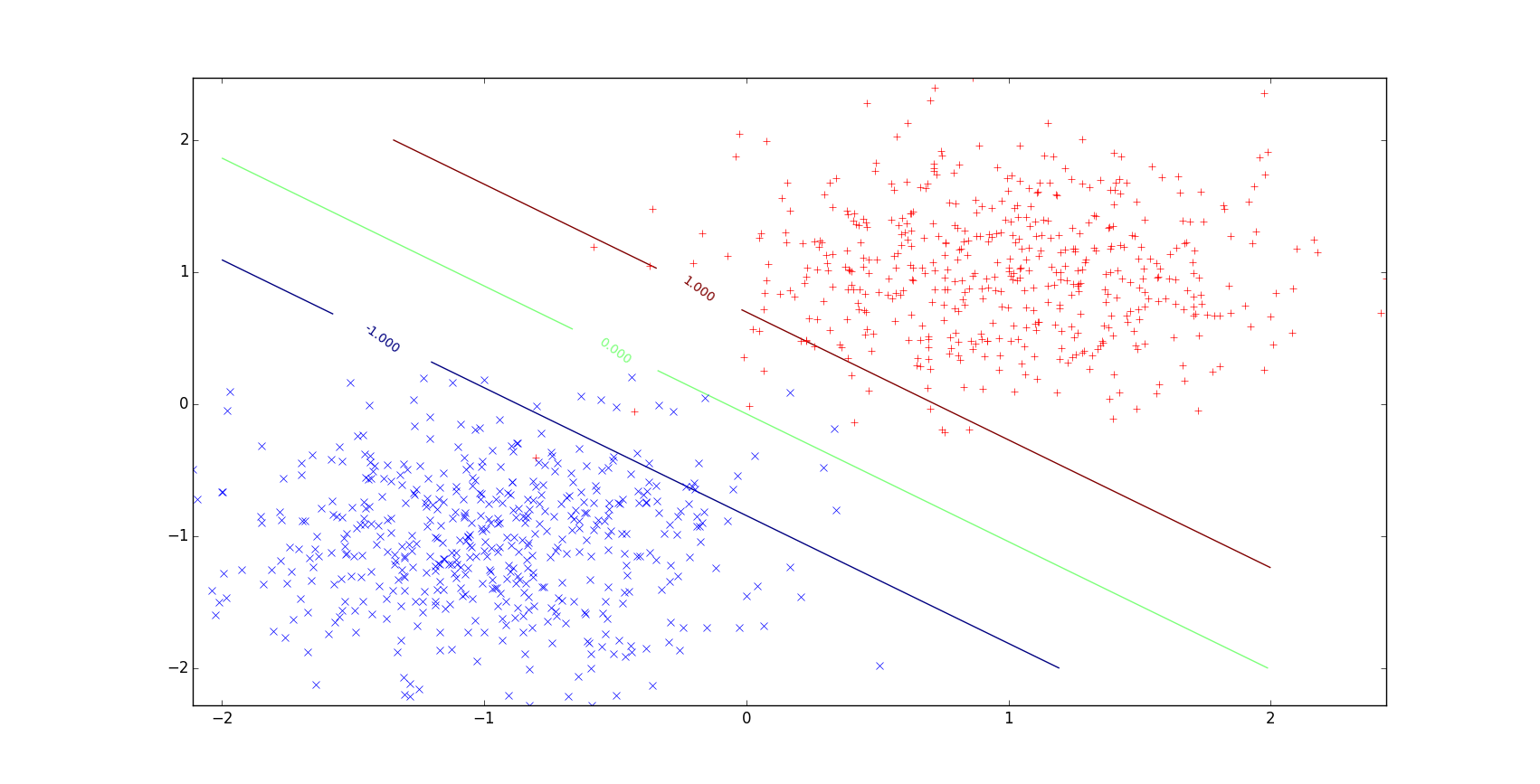
Figure 3: 2D linear

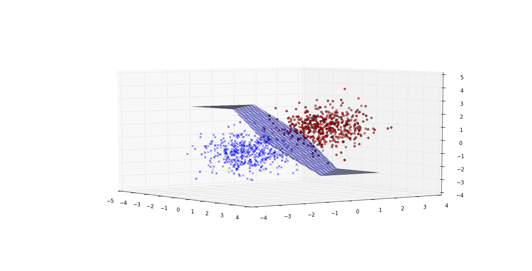
Figure 4: 3D linear

3.2 收敛速度

我们比较两种实现的收敛速度差异。这里，我们使用 5GB 带有 1000 个特征的模拟数据。使用 4 个 executors 并迭代 100 次。

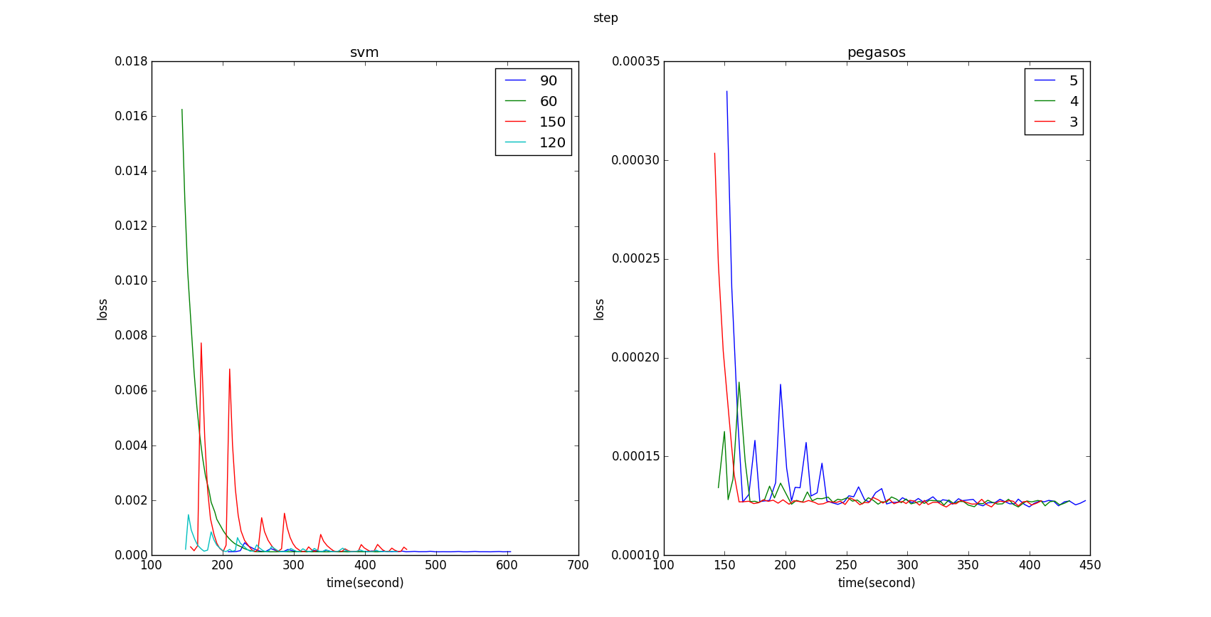
Figure 5: before aligning Y axis

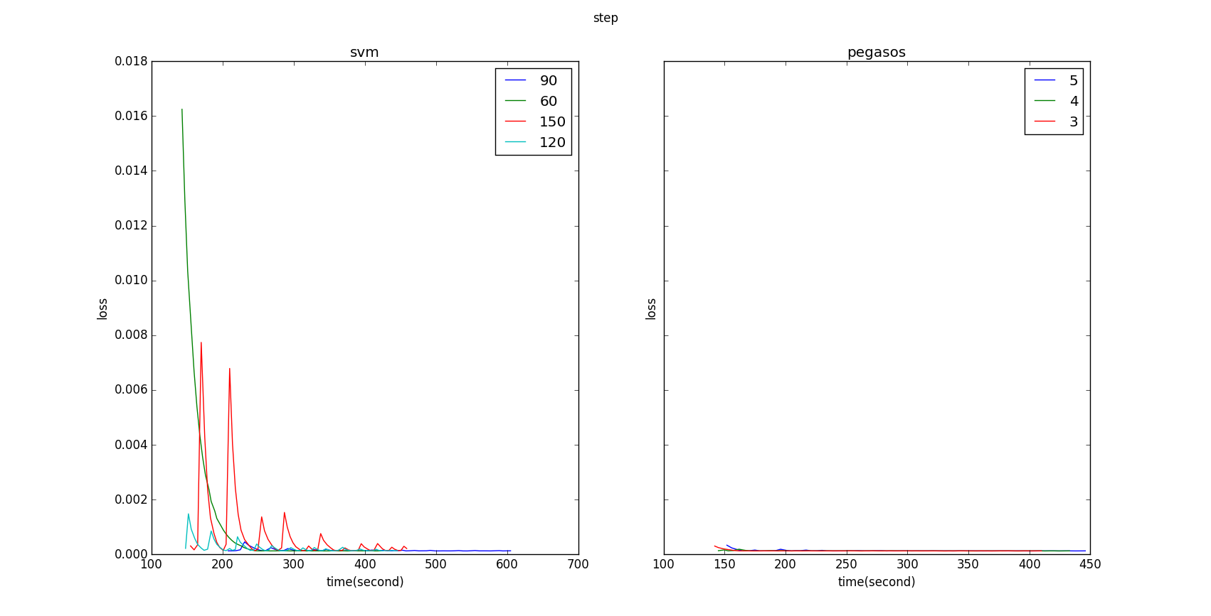
Figure 6: after aligning Y axis

4 参考文献

Zaharia, Matei, et al. "Resilient distributed datasets: A fault-tolerant abstraction for in-memory cluster computing." Proceedings of the 9th USENIX conference on Networked Systems Design and Implementation. USENIX Association, 2012
Zaharia, Matei, et al. "Spark: cluster computing with working sets." Proceedings of the 2nd USENIX conference on Hot topics in cloud computing. Vol. 10. 2010
Shalev-Shwartz, Shai, et al. "Pegasos: Primal estimated sub-gradient solver for svm." Mathematical programming 127.1 (2011): 3-30

Last Updated 2017-08-25 五 12:05.
Render by hexo-renderer-org with Emacs 24.5.1 (Org mode 8.2.10)